Max Weylandt.
← BackA null result: induced threat from immigration doesn’t seem to affect efficacy (a fair bit later in the survey)
28 December, 2023TL;DR
Ford and Mellon (2020) implemented a survey experiment in the European Social survey that should stimulate threat in respondents. Their outcome is support for immigration. While their experiment was at the end of the survey, the surveyors did test some new questions, responses to which could have presumably been affected by this treatment as well. While a bunch of questions measuring efficacy are statistically significant, the coefficients are basically zero.
Ford and Mellon’s paper
At the end of the European Social Survey, Ford and Mellon (2020) give people one of four immigrant profiles and ask them how many people of that group should be allowed to immigrate to the respondent’s country. The profiles differ on two axes: skill level (‘professionals’ vs ‘unskilled laborers’) and cultural proximity (these depended on country, but were often European vs non-European).
They frame this as the interplay between a skills premium and an ethnic premium. In a related corner of the literature, on group threat, we might talk about realistic threat (perceived threats to people’s economic or physical wellbeing) and symbolic threat (perceived threats to their cultural superiority) (Stephan, Ybarra, and Rios 2015).
Whatever you call it, they find that people prefer skilled migrants, and often (but not always) prefer Europeans over non-Europeans.
I learned about this paper from Claassen and McLaren (2021), which kind of puts forward the idea of correlating other attitudes with this experiment, which I thought was quite clever.
I then learned that this experiment was right at the end of the questionnaire. This makes sense – if seeing these profiles affects how people answer about immigration, it might affect other answers too, and so it’s best not to mess up other questions. Luckily for our purposes here the survey researchers did ask some questions afterwards, because they were testing some question wordings for inclusion in a future round. Not all of them are relevant, but I thought there might be a plausible story where raised level of threat affects people’s efficacy.
Measures
I had some choosing to do. Because these are test questions,they are asked a bunch of different ways, with respondents assigned one kind of question randomly. I wanted to choose one formulation each from the get go, to avoid (subconsciously) picking the most favourable one as data analysis went on.
I basically decided to use the question format they ended up using in round 8 for the survey – after all, they spent a lot of energy on deciding that one was the optimal way to ask for this attitude.
| Variable | Question | Scale |
|---|---|---|
| testf13 | How much would you say the political system in [country] allows people like you to have a say in what the government does? | 1 Not at all 2 Very little 3 Some 4 A lot 5 A great deal |
| testf14 | And how much would you say that the political system in [country] allows people like you to have an influence on politics? Please use the same card | 1 Not at all 2 Very little 3 Some 4 A lot 5 A great deal |
| testf15 | How much would you say that politicians care what people like you think? Please use the same card. | 1 Not at all 2 Very little 3 Some 4 A lot 5 A great deal |
| testf16 | How able do you think you are to take an active role in a group involved with political issues? Please use this card. | 1 Not at all able 2 A little able 3 Quite able 4 Very able 5 Completely able |
| testf17 | And using this card, how confident are you in your own ability to participate in politics? | 1 Not at all confident 2 A little confident 3 Quite confident 4 Very confident 5 Completely confident |
Details: Measures
The best file to follow all of this is perhaps the one called
ESS7_data_protocol_e01_2.pdf. I would link it but the links
I used are already dead, so I can’t trust the new ones staying live
either.
Data Preparation
I quickly tried to replicate their results, just to make sure that I had done the recoding right.
Details: Data import
 data <- read_dta("ESS7e02_2.stata/ESS7e02_2.dta")

data <- data %>% mutate(threat_econ = case_when(
  admaimg == 3 | admaimg == 4 ~ "low-skilled",
  admaimg == 1 | admaimg == 2 ~ "Professional",
  TRUE ~ NA_character_
  ),
  threat_cultural = case_when(
  admaimg == 1 | admaimg == 3 ~ "EU",
  admaimg == 4 | admaimg == 2 ~ ".Non-EU",
  TRUE ~ NA_character_
  )

  )

data <- data %>% mutate(Y = coalesce(alpfpe, alpfpne, allbpe, allbpne))

data <- data %>% mutate(Y_flipped = case_when(
  Y == 4 ~ 1,
  Y == 3 ~ 2,
  Y == 2 ~ 3,
  Y == 1 ~ 4,
  TRUE ~ NA_real_
))
Details: Model Replication
 # Run Replication


mod_pooled_fl <- lm(Y_flipped~  threat_cultural* threat_econ, data=data)

# Make Table

get_estimates(mod_pooled_fl)[,c(1:3,7,9)] %>%
  slice(2, 3:4, 1) %>%
  mutate(term = str_replace(term, "threat_culturalEU", "Ethnic Premium"),
         term = str_replace(term, "threat_econProfessional", "High skill premium"),
         term = str_replace(term, "Ethnic Premium:High skill premium", "Ethnic x high Skill")) %>%  kable(digits=c(0,2,3,2,3,3))
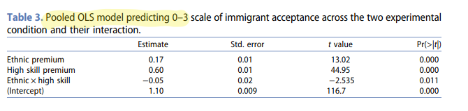
| term | estimate | std.error | statistic | p.value |
|---|---|---|---|---|
| Ethnic Premium | 0.17 | 0.013 | 13.02 | 0.000 |
| High skill premium | 0.60 | 0.013 | 44.95 | 0.000 |
| Ethnic x high Skill | -0.05 | 0.019 | -2.53 | 0.011 |
| (Intercept) | 2.10 | 0.009 | 222.81 | 0.000 |
Pooled models: efficacy ~ threat
So I joined in the supplemental data,and estimated five models: for each outcome, a simple linear regression of efficacy on the threat indicators, pooled across all countries.
Details: load and join supplementary data
 # load in supplementary data as data2
data2 <- read_dta("ESS7MTMMe02_1.stata/ESS7MTMMe2_1.dta")
data2 <- essurvey::recode_missings(data2)

#join it to the main survey
joined <- left_join(data, data2, by=c("cntry", "idno"))

# clone response columns to ones with legible names
joined <- joined %>%
  mutate(say_in_gov = testf13,
         influence_pol = testf14,
         pol_care = testf15,
         able_groups = testf16,
         able_particip = testf17)
Details: pooled model
 mod1 <- lm(say_in_gov ~ threat_cultural* threat_econ, data=joined)

mod2 <- lm(influence_pol ~ threat_cultural* threat_econ, data=joined)

mod3 <- lm(pol_care ~ threat_cultural* threat_econ, data=joined)

mod4 <- lm(able_groups ~ threat_cultural* threat_econ, data=joined)

mod5 <- lm(able_particip ~ threat_cultural* threat_econ, data=joined)


models <- list("System lets us have say"= mod1,
               "Can Influence Politics"= mod2,
               "Politicians Care" = mod3,
               "Able to take active role" = mod4,
               "Able to participate in politics" = mod5)
table_pooled <- sjPlot::tab_model(models,
                  show.ci = FALSE,
                  p.style = "stars")
|
Political system allows people to have a say in what government does |
Political system allows people to have influence on politics |
Politicians care what people think |
Able to take active role in political group |
Confident in own ability to participate in politics |
|
|---|---|---|---|---|---|
| Predictors | Estimates | Estimates | Estimates | Estimates | Estimates |
| (Intercept) | 2.27 *** | 2.22 *** | 2.17 *** | 2.09 *** | 2.10 *** |
| threat cultural [EU] | 0.04 | 0.04 * | 0.06 ** | 0.02 | 0.02 |
|
threat econ [Professional] |
0.03 | -0.01 | -0.03 | -0.02 | -0.03 |
|
threat cultural [EU] × threat econ [Professional] |
0.01 | 0.00 | -0.00 | 0.02 | 0.05 |
| Observations | 19420 | 19450 | 19511 | 19398 | 19414 |
| R2 / R2 adjusted | 0.001 / 0.001 | 0.001 / 0.000 | 0.001 / 0.001 | 0.000 / 0.000 | 0.001 / 0.000 |
| * p<0.05 ** p<0.01 *** p<0.001 | |||||
so, not much going at all. This is the same models with country fixed effects:
Details: fixed effects model
Note that below I interact the country dummies with the treatments. In my view it’s plausible that the treatments work differently in different countries. I later found that this yields the ‘strongest’ effects (in inverted commas because they’re still basically nulls imo) – if I run models where the country-level variable doesn’t influence the treatment variables, the coefficients are all between 0 and 0.02.
 mod1 <- lm(say_in_gov ~ threat_cultural* threat_econ * factor(cntry) , data=joined)

mod2 <- lm(influence_pol ~ threat_cultural* threat_econ * factor(cntry), data=joined)

mod3 <- lm(pol_care ~ threat_cultural* threat_econ * factor(cntry), data=joined)

mod4 <- lm(able_groups ~ threat_cultural* threat_econ * factor(cntry), data=joined)

mod5 <- lm(able_particip ~ threat_cultural* threat_econ * factor(cntry), data=joined)


models <- list("System lets us have say"= mod1,
               "Can Influence Politics"= mod2,
               "Politicians Care" = mod3,
               "Able to take active role" = mod4,
               "Able to participate in politics" = mod5)
table_fe <-sjPlot::tab_model(models,
                  show.ci = FALSE,
                  p.style = "stars")
|
Political system allows people to have a say in what government does |
Political system allows people to have influence on politics |
Politicians care what people think |
Able to take active role in political group |
Confident in own ability to participate in politics |
|
|---|---|---|---|---|---|
| Predictors | Estimates | Estimates | Estimates | Estimates | Estimates |
| (Intercept) | 2.34 *** | 2.35 *** | 2.11 *** | 2.51 *** | 2.56 *** |
| threat_culturalEU | -0.06 | -0.08 | 0.01 | -0.21 * | -0.23 * |
| threat_econProfessional | -0.11 | -0.15 | -0.06 | -0.12 | -0.21 * |
| factor(cntry)BE | 0.04 | -0.07 | 0.19 * | -0.66 *** | -0.67 *** |
| factor(cntry)CH | 0.82 *** | 0.63 *** | 0.70 *** | -0.17 | -0.04 |
| factor(cntry)CZ | 0.02 | -0.18 * | 0.01 | -0.56 *** | -0.75 *** |
| factor(cntry)DE | 0.12 | 0.12 | 0.16 * | -0.32 *** | -0.05 |
| factor(cntry)DK | 0.41 *** | 0.53 *** | 0.51 *** | 0.26 * | 0.04 |
| factor(cntry)EE | -0.34 *** | -0.44 *** | -0.06 | -0.70 *** | -0.80 *** |
| factor(cntry)ES | -0.30 *** | -0.44 *** | -0.26 *** | -0.63 *** | -0.52 *** |
| factor(cntry)FI | -0.16 * | 0.02 | 0.32 *** | -0.20 * | -0.41 *** |
| factor(cntry)FR | -0.09 | -0.24 ** | -0.07 | -0.71 *** | -0.30 ** |
| factor(cntry)GB | -0.11 | -0.24 ** | 0.09 | -0.32 *** | -0.41 *** |
| factor(cntry)HU | -0.35 *** | -0.46 *** | -0.22 ** | -0.63 *** | -0.81 *** |
| factor(cntry)IE | -0.23 ** | -0.20 * | -0.03 | -0.32 *** | -0.42 *** |
| factor(cntry)IL | -0.36 *** | -0.35 *** | -0.14 | -0.57 *** | -0.67 *** |
| factor(cntry)LT | -0.20 * | -0.44 *** | -0.07 | -0.60 *** | -0.66 *** |
| factor(cntry)NL | 0.38 *** | 0.21 ** | 0.53 *** | -0.57 *** | -0.75 *** |
| factor(cntry)NO | 0.41 *** | 0.54 *** | 0.58 *** | 0.06 | -0.08 |
| factor(cntry)PL | -0.01 | -0.41 *** | -0.32 *** | -0.59 *** | -0.65 *** |
| factor(cntry)PT | -0.31 ** | -0.40 *** | -0.36 *** | -0.78 *** | -0.93 *** |
| factor(cntry)SE | 0.49 *** | 0.45 *** | 0.56 *** | -0.08 | -0.15 |
| factor(cntry)SI | -0.67 *** | -0.65 *** | -0.44 *** | -0.63 *** | -0.67 *** |
| threat_culturalEU:threat_econProfessional | 0.19 | 0.18 | 0.07 | 0.21 | 0.24 |
| threat_culturalEU:factor(cntry)BE | 0.07 | 0.11 | 0.10 | 0.24 | 0.20 |
| threat_culturalEU:factor(cntry)CH | 0.07 | 0.04 | -0.13 | 0.22 | 0.35 * |
| threat_culturalEU:factor(cntry)CZ | 0.12 | 0.09 | 0.05 | 0.17 | 0.32 * |
| threat_culturalEU:factor(cntry)DE | -0.03 | 0.07 | -0.09 | 0.22 | 0.27 * |
| threat_culturalEU:factor(cntry)DK | 0.17 | 0.12 | 0.04 | 0.21 | 0.29 |
| threat_culturalEU:factor(cntry)EE | 0.12 | 0.19 | 0.06 | 0.27 * | 0.26 |
| threat_culturalEU:factor(cntry)ES | -0.17 | -0.16 | -0.29 | -0.29 | -0.39 |
| threat_culturalEU:factor(cntry)FI | 0.14 | 0.13 | 0.09 | 0.13 | 0.08 |
| threat_culturalEU:factor(cntry)FR | -0.07 | -0.05 | -0.00 | 0.49 *** | 0.37 ** |
| threat_culturalEU:factor(cntry)GB | 0.11 | 0.17 | 0.02 | 0.19 | 0.30 * |
| threat_culturalEU:factor(cntry)HU | -0.11 | -0.09 | -0.12 | 0.11 | 0.08 |
| threat_culturalEU:factor(cntry)IE | 0.06 | 0.05 | -0.12 | 0.14 | 0.21 |
| threat_culturalEU:factor(cntry)IL | 0.08 | -0.00 | -0.06 | 0.27 * | 0.39 ** |
| threat_culturalEU:factor(cntry)LT | 0.03 | 0.13 | -0.02 | 0.22 | 0.24 |
| threat_culturalEU:factor(cntry)NL | -0.06 | 0.06 | -0.02 | -0.05 | 0.09 |
| threat_culturalEU:factor(cntry)NO | 0.11 | -0.01 | 0.08 | 0.26 | 0.14 |
| threat_culturalEU:factor(cntry)PL | -0.03 | 0.13 | 0.04 | 0.19 | 0.33 * |
| threat_culturalEU:factor(cntry)PT | 0.03 | 0.06 | -0.07 | 0.22 | 0.27 |
| threat_culturalEU:factor(cntry)SE | -0.10 | -0.03 | -0.11 | 0.29 * | 0.27 |
| threat_econProfessional:factor(cntry)BE | 0.12 | 0.15 | 0.11 | 0.24 | 0.27 |
| threat_econProfessional:factor(cntry)CH | 0.02 | 0.08 | -0.13 | 0.10 | 0.30 * |
| threat_econProfessional:factor(cntry)CZ | 0.04 | 0.13 | -0.05 | 0.06 | 0.19 |
| threat_econProfessional:factor(cntry)DE | 0.18 | 0.21 * | 0.03 | 0.11 | 0.18 |
| threat_econProfessional:factor(cntry)DK | 0.22 | 0.19 | 0.17 | 0.14 | 0.29 |
| threat_econProfessional:factor(cntry)EE | 0.18 | 0.22 * | 0.12 | 0.06 | 0.19 |
| threat_econProfessional:factor(cntry)ES | 0.17 | 0.26 * | 0.08 | 0.12 | 0.16 |
| threat_econProfessional:factor(cntry)FR | 0.00 | 0.07 | 0.06 | 0.21 | 0.16 |
| threat_econProfessional:factor(cntry)GB | 0.20 | 0.29 * | 0.05 | 0.21 | 0.31 * |
| threat_econProfessional:factor(cntry)HU | 0.10 | 0.07 | -0.05 | 0.17 | 0.16 |
| threat_econProfessional:factor(cntry)IE | 0.13 | 0.10 | -0.04 | 0.15 | 0.14 |
| threat_econProfessional:factor(cntry)IL | 0.24 * | 0.19 | 0.07 | 0.35 ** | 0.29 * |
| threat_econProfessional:factor(cntry)LT | 0.11 | 0.21 | 0.07 | 0.09 | 0.20 |
| threat_econProfessional:factor(cntry)NL | 0.04 | 0.11 | 0.06 | -0.12 | 0.08 |
| threat_econProfessional:factor(cntry)NO | 0.25 | 0.16 | 0.18 | 0.20 | 0.26 |
| threat_econProfessional:factor(cntry)PL | 0.13 | 0.12 | 0.04 | 0.01 | 0.13 |
| threat_econProfessional:factor(cntry)PT | 0.31 * | 0.21 | 0.18 | 0.18 | 0.18 |
| threat_econProfessional:factor(cntry)SE | 0.02 | 0.14 | 0.11 | 0.30 * | 0.34 * |
| threat_econProfessional:factor(cntry)SI | 0.19 | 0.13 | 0.06 | 0.07 | 0.14 |
| threat_culturalEU:threat_econProfessional:factor(cntry)BE | -0.31 | -0.30 | -0.24 | -0.29 | -0.27 |
| threat_culturalEU:threat_econProfessional:factor(cntry)CH | -0.08 | -0.05 | 0.10 | -0.29 | -0.36 |
| threat_culturalEU:threat_econProfessional:factor(cntry)CZ | -0.14 | -0.22 | -0.08 | -0.08 | -0.24 |
| threat_culturalEU:threat_econProfessional:factor(cntry)DE | -0.20 | -0.20 | 0.01 | -0.25 | -0.24 |
| threat_culturalEU:threat_econProfessional:factor(cntry)DK | -0.47 * | -0.31 | -0.30 | -0.43 * | -0.58 ** |
| threat_culturalEU:threat_econProfessional:factor(cntry)EE | -0.23 | -0.29 | -0.23 | -0.22 | -0.27 |
| threat_culturalEU:threat_econProfessional:factor(cntry)ES | 0.15 | 0.00 | 0.25 | 0.05 | 0.13 |
| threat_culturalEU:threat_econProfessional:factor(cntry)FR | -0.11 | -0.17 | -0.20 | -0.54 ** | -0.32 |
| threat_culturalEU:threat_econProfessional:factor(cntry)GB | -0.19 | -0.29 | -0.06 | -0.26 | -0.29 |
| threat_culturalEU:threat_econProfessional:factor(cntry)HU | -0.03 | 0.03 | 0.08 | -0.19 | -0.14 |
| threat_culturalEU:threat_econProfessional:factor(cntry)IE | -0.20 | -0.13 | 0.09 | -0.17 | -0.15 |
| threat_culturalEU:threat_econProfessional:factor(cntry)IL | -0.35 * | -0.15 | -0.00 | -0.42 * | -0.35 |
| threat_culturalEU:threat_econProfessional:factor(cntry)LT | -0.21 | -0.31 * | -0.18 | -0.24 | -0.25 |
| threat_culturalEU:threat_econProfessional:factor(cntry)NL | -0.09 | -0.22 | -0.18 | 0.32 | 0.05 |
| threat_culturalEU:threat_econProfessional:factor(cntry)NO | -0.34 | -0.13 | -0.10 | -0.28 | -0.12 |
| threat_culturalEU:threat_econProfessional:factor(cntry)PL | -0.26 | -0.36 * | -0.22 | -0.04 | -0.20 |
| threat_culturalEU:threat_econProfessional:factor(cntry)PT | -0.28 | -0.19 | -0.04 | -0.27 | -0.17 |
| threat_culturalEU:threat_econProfessional:factor(cntry)SE | 0.01 | -0.08 | -0.01 | -0.45 * | -0.47 * |
| Observations | 19420 | 19450 | 19511 | 19398 | 19414 |
| R2 / R2 adjusted | 0.106 / 0.102 | 0.135 / 0.132 | 0.118 / 0.115 | 0.063 / 0.059 | 0.076 / 0.072 |
| * p<0.05 ** p<0.01 *** p<0.001 | |||||
Individual Country Regressions
Ok, so there are a few results significant at the .05 level – still not much to write home about imo. Here are some regressions of the outcomes on the interaction of the two threats for each country, only showing the coefficients for culture.
Details: individual country plots
 countries <- unique(joined$cntry)

variables <- c("say_in_gov", "influence_pol", "pol_care", "able_groups", "able_particip")

outcomes <- data.frame(country_test = countries,
                       country=NA,
                       coef = NA,
                       se = NA,
                       ci_low = NA,
                       ci_high = NA )

# remove SI and FI
# those who got EU in SI or Professional in FI didn't get
# asked the outcome variables (or they are NA for another reason)

countries <- countries[-c(9,21)]

graphs <- list()

for (v in 1:length(variables)) {

  for (i in 1:length(countries)) {
    data_filtered <- joined %>% filter(cntry==countries[i])

    mod <- lm(as.formula(paste(variables[v], "~ threat_cultural * threat_econ")) , data=data_filtered)

    estimates <- get_estimates(mod)

    outcomes$country[i] = countries[i]
    outcomes$coef[i]    = estimates$estimate[2]
    outcomes$se[i]      = estimates$std.error[2]
    outcomes$ci_low[i]  = estimates$conf.low[2]
    outcomes$ci_high[i] = estimates$conf.high[2]


    p <- ggplot(outcomes) +
      aes(x=reorder(country,coef), y=coef) +
      geom_point() +
      geom_segment(aes(x=country,xend=country, y=ci_low, yend=ci_high   ))+
      geom_hline(yintercept=0, color="grey")+
      labs(x = "Country", y="Effect of Cultural Threat", title = variables[v])+
      theme_bw()+
      theme(text = element_text(size=8))+
      ylim(c(-0.5, 1))

    graphs[[v]] <- p

  }
}

graphs[[1]] + graphs[[2]] + graphs[[3]]
graphs[[5]] + graphs[[4]]
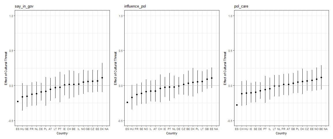
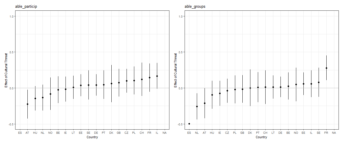
As far as I’m concerned there’s nothing here.
Placebo Analysis
Because I had planned to do so anyways, I did go ahead and ran a placebo test where I regressed other survey questions that I thought would be unrelated. They should be, because they came before the treatment. Indeed the effects are null.
|
Qualification for immigration:committed to way of life in country |
Trust in politicians |
Belonging to particular religion or denomination |
|
|---|---|---|---|
| Predictors | Estimates | Estimates | Estimates |
| (Intercept) | 7.35 *** | 3.55 *** | 1.42 *** |
| threat cultural [EU] | 0.01 | 0.01 | 0.01 |
|
threat econ [Professional] |
0.03 | 0.05 | 0.01 |
|
threat cultural [EU] × threat econ [Professional] |
-0.04 | -0.05 | -0.01 |
| Observations | 39652 | 39666 | 40002 |
| R2 / R2 adjusted | 0.000 / -0.000 | 0.000 / -0.000 | 0.000 / -0.000 |
| * p<0.05 ** p<0.01 *** p<0.001 | |||
Conclusion
So, I didn’t find any effects of this threat treatment on a bunch of efficacy measures.
This was a very brief analysis and there are lots of other things you could do, including looking at the people who were asked other versions of the efficacy questions. After all, I only looked at the subset that was randomly assigned to see these particular formulations. I’m sure there’s also lots you could do on the modeling side. And, for sure, there was quite the gap between the treatment and when they were asked about efficacy (there was lots of demographic info in the middle). So maybe this relationship does exist in real life. But in this dataset? I doubt it. I tend to think that if the effect is there a simple analysis should find it.
Cited
← Back ↑ Top